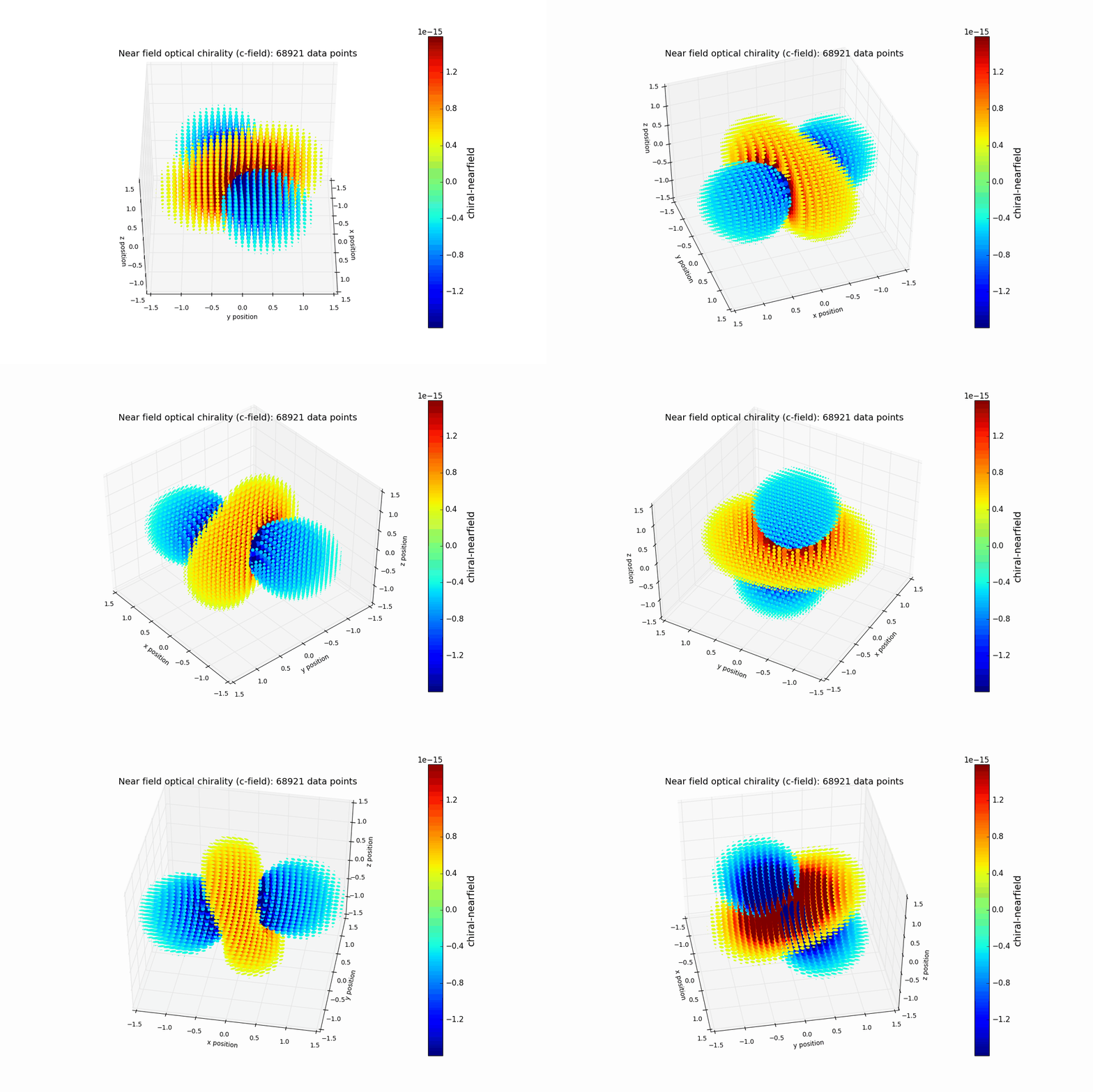
Near-field optical chirality by electric dipoles

Created: 22 April 2017

The code was originally written in June 2016.

Near-field optical chirality

Optical chirality comes in forms of circular polarizations: left-handed or right-handed. Achiral light i.e. linearly polarized light can gain optical chirality through interacting with chiral media such as chiral molecules. The effect can be observed with techniques such as circular dichroism spectroscopy

Although not being able to induce far-field chirality to light, a symmetric optical antenna can create localized field of optical chirality.

Calculating chiral near-field

The following code calculates and plots 3-dimensional distribution of chiral optical near-field generated by two orthogonal electric dipoles when excited by an electromagnetic field.

Two categories of the incident field can be used:

Linearly polarized
Elliptically polarized with \(E_y\) has 90deg phase lag with respect to \(E_x\).

In both cases, the relative magnitude of \(E_x\) and \(E_y\) can be adjusted by changing the angle \(\psi\) (psi), with respect to the x-axis i.e. \(E_x\sim\cos(\psi)\) and \(E_y\sim\sin(\psi)\).

The code was developed based on two articles: M. Schaferling, OptEx 2012 and T. J. Davis, PhyRevB 2013.

Import libraries

The chital_local function is home-written and is provided here.

%matplotlib notebook

import numpy as np
from mpl_toolkits.mplot3d import Axes3D
import matplotlib.pyplot as plt

# the function excludes intrinsic chiral field from the incident field
from chiral_local import chiral_local

Set parameters for the incident electromagnetic field

The necessary parameters are passed to the calculation as incWave.

# define the incident electric field's parameters

freq = 500e12              # set the frequency of the incident field e.g. 500 THz (600nm wavelength)
omega = 2*np.pi*freq
c = 3e8                    # speed of light in m/s
k = omega/c               
psiDeg = -45               # e.g. set psiDeg=45 to have |E_x|=|E_y|, changing the sign (+ or -) results in changing the handedness when using an elliptically incident field
psi = psiDeg/180*np.pi

incWave=[k, psi]

Define parameters for two electric dipoles

\(p_x\) and \(p_y\) are the strength, \(A_x\) and \(A_y\) are constants that depend on the plasma frequency, \(\omega_{res,x}\) and \(\omega_{res,y}\) are the resonance frequencies, and \(\Gamma_x\) and \(\Gamma_y\) are the loss terms of the dipoles. For more details, please find the notions in T. J. Davis, PhyRevB 2013.

For simplicity, the y-dipole is set to zero in this example. The resulting plot resembles what shown in Figure 2 of T. J. Davis, PhyRevB 2013.

## define parameters

# x-dipole
p_x = 1
A_x = 1
omegaRes_x = omega
Gamma_x = 0.5*omegaRes_x
deltaOmega_x = omega - omegaRes_x
beta_x = A_x*p_x**2/(deltaOmega_x**2 + Gamma_x**2/4)
xDipole = [beta_x,Gamma_x,deltaOmega_x]

# y-dipole
p_y = 0
A_y = 1*A_x
omegaRes_y = omega
Gamma_y = 0.1*omegaRes_y
deltaOmega_y = omega - omegaRes_y
beta_y = A_y*p_y**2/(deltaOmega_y**2 + Gamma_y**2/4)
yDipole = [beta_y,Gamma_y,deltaOmega_y]

Set plot volume

## set plot volume

[xlim, ylim, zlim] = [2, 2, 2]
[nx, ny, nz] = [41, 41, 41]

x,y,z = np.meshgrid(np.linspace(-xlim,xlim,nx), np.linspace(-ylim,ylim,ny), np.linspace(-zlim,zlim,nz))
x = x.flatten()
y = y.flatten()
z = z.flatten()

r = np.sqrt(x**2 + y**2 + z**2)

# define position in a spherical coordinate (r, tetha, phi)
position=[r, np.arcsin(z/r), np.arctan2(y,x)]

Calculate localized optical chiral field, make sure to select the correct mode!

# perform calculation

c_local = np.zeros_like(position[0])
mode = 'linear'

for i in range(position[0].size):
    pos = [position[0][i],position[1][i],position[2][i]]
    c_local[i] = chiral_local(incWave, xDipole, yDipole, pos, mode)    

3D interactive plot in ipython/Jupyter notebook

# plot

scale=omega
colorLim = 5/omega

fig = plt.figure(figsize=(12,8))
ax = fig.add_subplot(111, projection='3d')
s_set = 150*np.log10((np.abs(c_local*omega)))    # scale the size of scatter points to improve visibility, note the log scale
p = ax.scatter(x, y, z, c=c_local, edgecolor=(0,0,0,0), s=s_set, cmap='jet', vmin=-colorLim, vmax=colorLim, depthshade=False)
fig.colorbar(p).set_label('chiral-nearfield', fontsize=15)

# axis labels
title_set = ('Near field optical chirality (c-field): ' + str(c_local.size) + ' data points')
ax.set_title(title_set, fontsize = 14)
ax.set_xlabel('x position', fontsize=10)
ax.set_ylabel('y position', fontsize=10)
ax.set_zlabel('z position', fontsize=10)
ax.tick_params(labelsize=10)

# axis limits
boxlim = 1.5
ax.set_xlim([-boxlim,boxlim])
ax.set_ylim([-boxlim,boxlim])
ax.set_zlim([-boxlim,boxlim])

# set initial viewing angles in degree
ax.view_init(elev=45, azim=45)