Basic stock analysis: requesting and plotting data

Created: 19 April 2017

Visualizing historical stock data

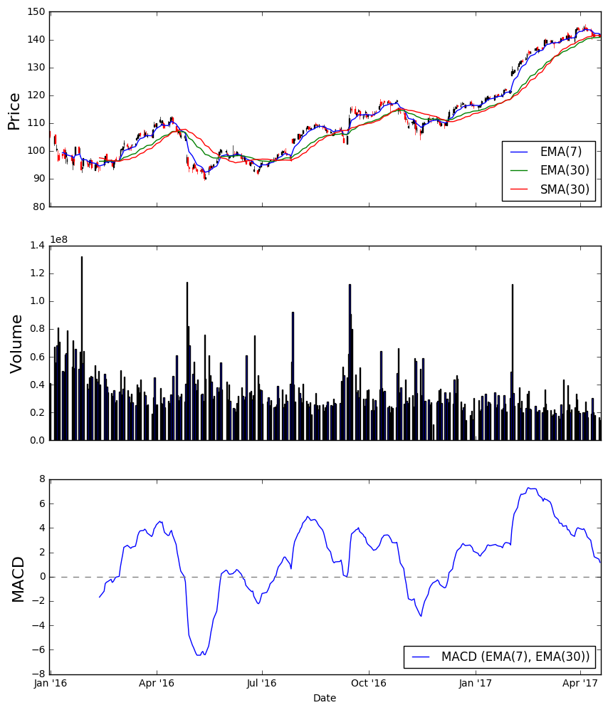
The following code shows how to get historical data of a stock from Google Finance (or Yahoo Finance) and plot a candlestick chart with simple moving average (SMA), exponential moving average (EMA), and Moving Average Convergence Divergence (MACD).

The code is an expansion of an answer in this Stack Overflow thread.

The code is written in python 3.5.2.

# import necessary libraries

%matplotlib inline  

import pandas_datareader.data as web
import pandas as pd
import matplotlib.pyplot as plt
from matplotlib import dates as mdates
from matplotlib.finance import candlestick_ohlc
import datetime as dt

Getting data from web

# request and reformat data

symbol = "AAPL"
data = web.DataReader(symbol, 'google', '2015-12-31', end = dt.datetime.now())  # use 'google' or 'yahoo' to pick the data source
data.reset_index(inplace=True)
data['Date']=mdates.date2num(data['Date'].astype(dt.date))

Define moving average models to plot

# setup moving average models

x = data['Date']

EMA_1_span = 7
EMA_1 = data['Close'].ewm(span=EMA_1_span,min_periods=EMA_1_span).mean()

EMA_2_span = 30
EMA_2 = data['Close'].ewm(span=EMA_2_span,min_periods=EMA_2_span).mean()

SMA_2_span = EMA_2_span
SMA_2 = data['Close'].rolling(window=SMA_2_span,center=False).mean()

MACD = EMA_1 - EMA_2

Plot stock data

# plot

fig, (ax, ax2, ax3) = plt.subplots(3, sharex=True, figsize=(10,12))

# plot candlestick, SAM, EMA in subplot_1
candlestick_ohlc(ax,data.values,width=0.5);
p1 = ax.plot(x, EMA_1, label='EMA(' + str(EMA_1_span) + ')')
p2 = ax.plot(x, EMA_2, label='EMA(' + str(EMA_2_span) + ')')
p3 = ax.plot(x, SMA_2, label='SMA(' + str(SMA_2_span) + ')')
ax.xaxis.set_major_formatter(mdates.DateFormatter('%Y-%m-%d'))
ax.xaxis.set_major_locator(mdates.MonthLocator([1,4,7,10]))
ax.xaxis.set_major_formatter(mdates.DateFormatter("%b '%y"))
ax.set_ylabel('Price', fontsize=16)
ax.legend(loc=4)

# plot volume in subplot_2
ax2.bar(x,data['Volume']);
ax2.set_ylabel('Volume', fontsize=16)

# plot MACD in subplot_3
ax3.plot(x, MACD, label='MACD (' + 'EMA(' + str(EMA_1_span) + '), ' + 'EMA(' + str(EMA_2_span) + '))')
ax3.axhline(0, color='gray', linestyle='--')
ax3.set_xlabel('Date')
ax3.set_ylabel('MACD', fontsize=16)
ax3.legend(loc=4)

Obtaining real-time stock price from Google Finance

The code below shows how to get real-time data of a stock from Google Finance page.

It is a modified version of files from this Github repository.

# import libraries

import urllib.request, time, re

Create a function to call stock data from Google Finance

# define data acquisition function

def fetchGF(googleticker):

    url = "http://www.google.com/finance?&q="
    respData = urllib.request.urlopen(url+ticker).read()

    # search for the tag with ref id of the stock and get the displayed price and currency
    price=re.search(b'id="ref_(.*?)">(.*?)<', respData)
    currency=re.search(b'Currency in (.*?)<', respData)

    if price:
        # get the price and re-format displayed text
        # group 1: ref id of the stock in the html page, group 2: price
        tmp=price.group(2)
        q=tmp.decode().replace(',','') + ' ' + currency.group(1).decode()
    else:
        q="Nothing found for: "+ googleticker

    return q

Call and display real-time price of a selected stock

# pick stock and display the current price
ticker = 'NASDAQ:GOOG'

print('As of '+ time.ctime() + ' local time, the price of ' + ticker + ' is ' + fetchGF(ticker) + '.')

As of Wed Apr 19 16:24:20 2017 local time, the price of NASDAQ:GOOG is 841.01 USD.

Closing note

The codes above show basic of requesting historical and real-time stock data as well as plotting charts/indicators. With some effort, the process could be made less tedious and more automated.